1 Classifiers#
Or: What is a chair?

Motivation#
Aristotelian Essentialism#
Let’s say we want to classify things in chairs and non-chairs. Wouldn’t it be helpful to first answer the question: What is a chair? Aristotelian essentialism is the philosophical view that entities possess an intrinsic essence that defines what they are. According to Aristotle, every object or being has a set of necessary properties that make it what it is and distinguish it from what it is not.
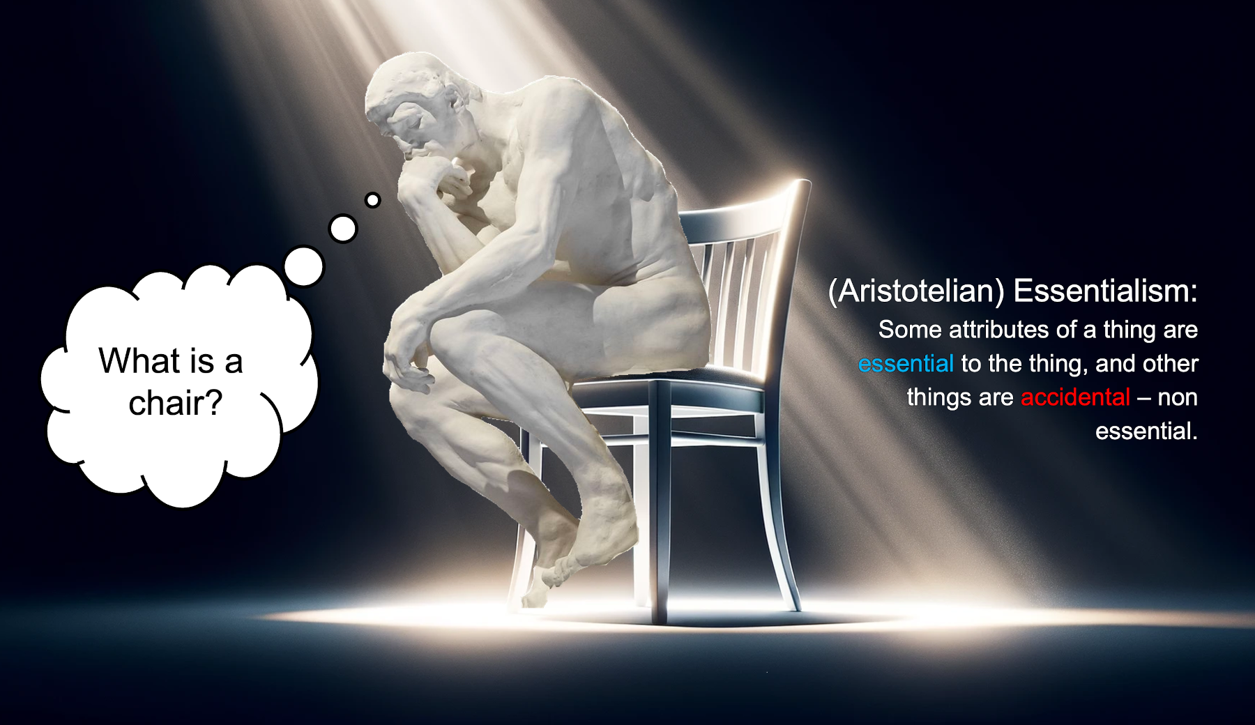
So, let’s define a chair this way:
A chair is has four legs and one can sit on it.
Is this definition helpful?


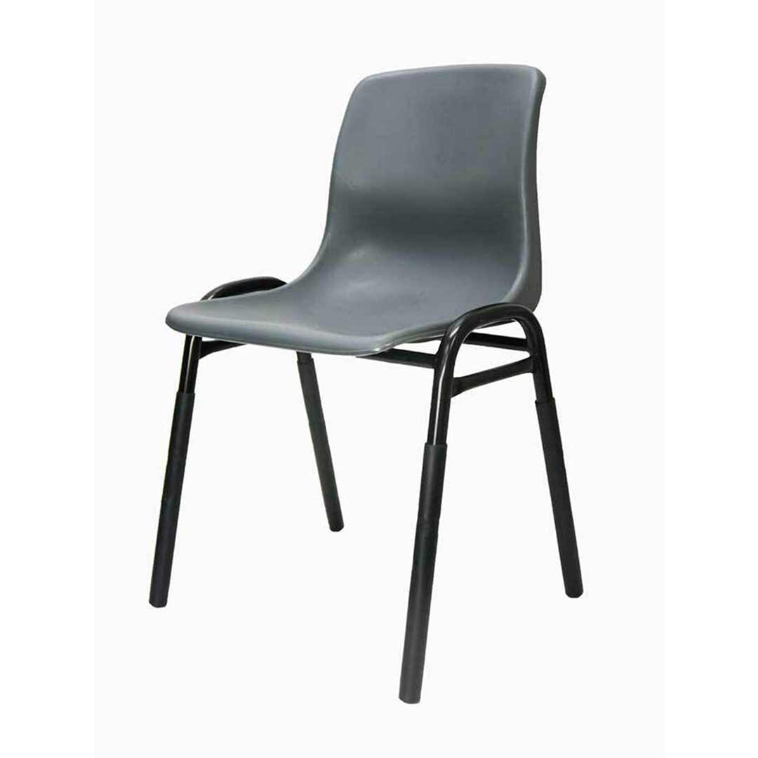

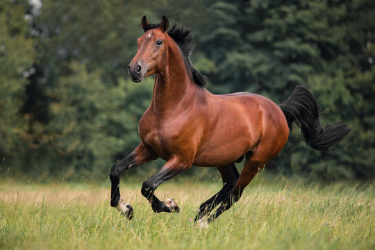
A horse has four legs and one can sit on it but a horse is not a chair!
Can we revise our definition?
A chair is nonliving, has four legs, and one can sit on it.

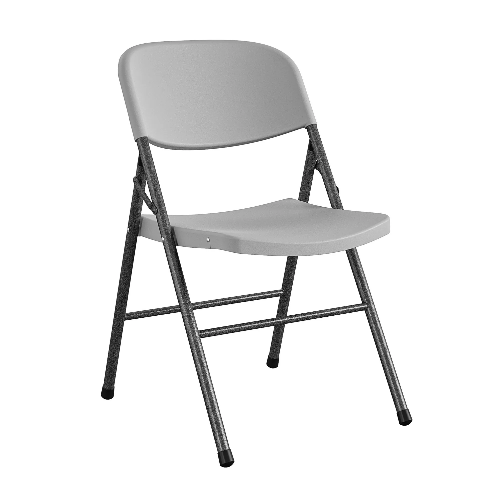


Some chairs have four legs, some have five. Some have three and there are even chairs without legs. The number of legs doesn’t seem to be essential to the definition of a chair.

Classification is Effortless!#
There appears to be a puzzle here. Have you ever mistaken a horse for a chair? If you encountered someone who made such an error, even just once, what advice would you give them?
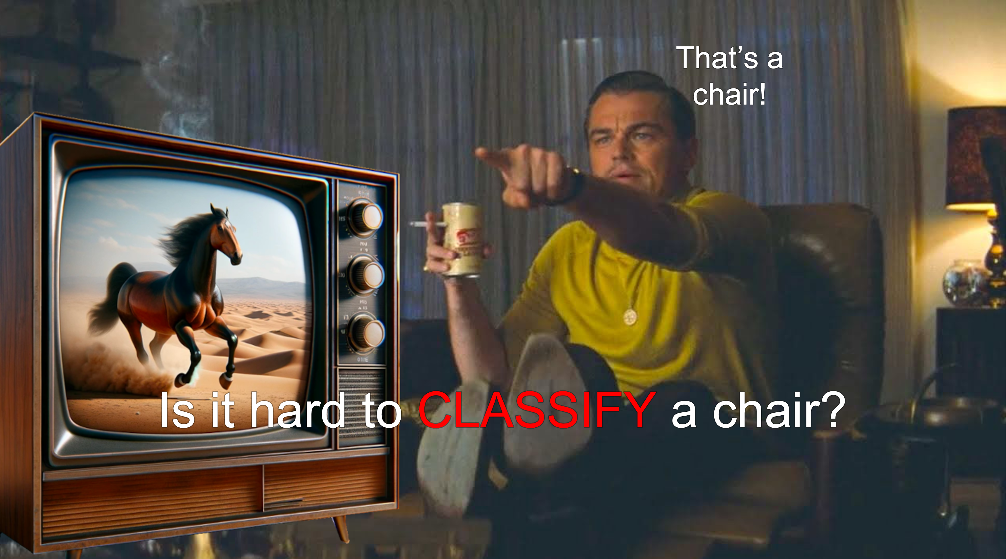
A neurologist would probably diagnose such a person with visual object agnosia. People seem to classify objects effortless. Remarkably, this ability develops naturally—after all, when was the last time you attended chair-class?

Machine Learning in a nutshell#
Directly writing a classifier function seems helpless:
def is_chair(object):
    """
    Returns True if something is a chair.
    """
    if has_legs(object):
        if nr_legs(object) == 4:
            if has_flat_surface(object):
                if is_stable(object):
                    if has_backrest(object):
                        if is_comforable_height(object):
                            if material(object) == 'wood':
                                ...
def has_legs(object):
    """
    Returns true if something has legs.
    """
    for element in object.elements:
        if is_leg(element):
            return true

def is_leg(object):
    """
    Returns true if something is a leg.
    """
    if is_attached_to(object, objects_that_have_legs):
        ...
Instead of directly writing a function that recognizes a chair, we write an algorithm that learns from data to create a function that recognizes a chair.
Classifying Classifiers#
To not get lost in the broader landscape of machine learning, we can think about different approaches in terms of key aspects. These include the type of data they process, the solution space that is considered, the learning algorithm employed, and the methods used to evaluate the resulting function.
It is important to note that all of these aspects are, to some extent, design choices. While “machine learning” is often perceived as a general-purpose tool that can be applied to almost any problem, its effectiveness depends on careful design decisions.
The art of machine learning involves:
Choosing an appropriate feature representation (i.e., organizing data effectively),
Defining a suitable solution space (i.e., constraining the problem appropriately),
Designing a meaningful loss function (i.e., determining how to evaluate solutions), and
Selecting an appropriate learning algorithm (e.g., formulating the problem as an optimization task to leverage general-purpose optimization methods).
Data#
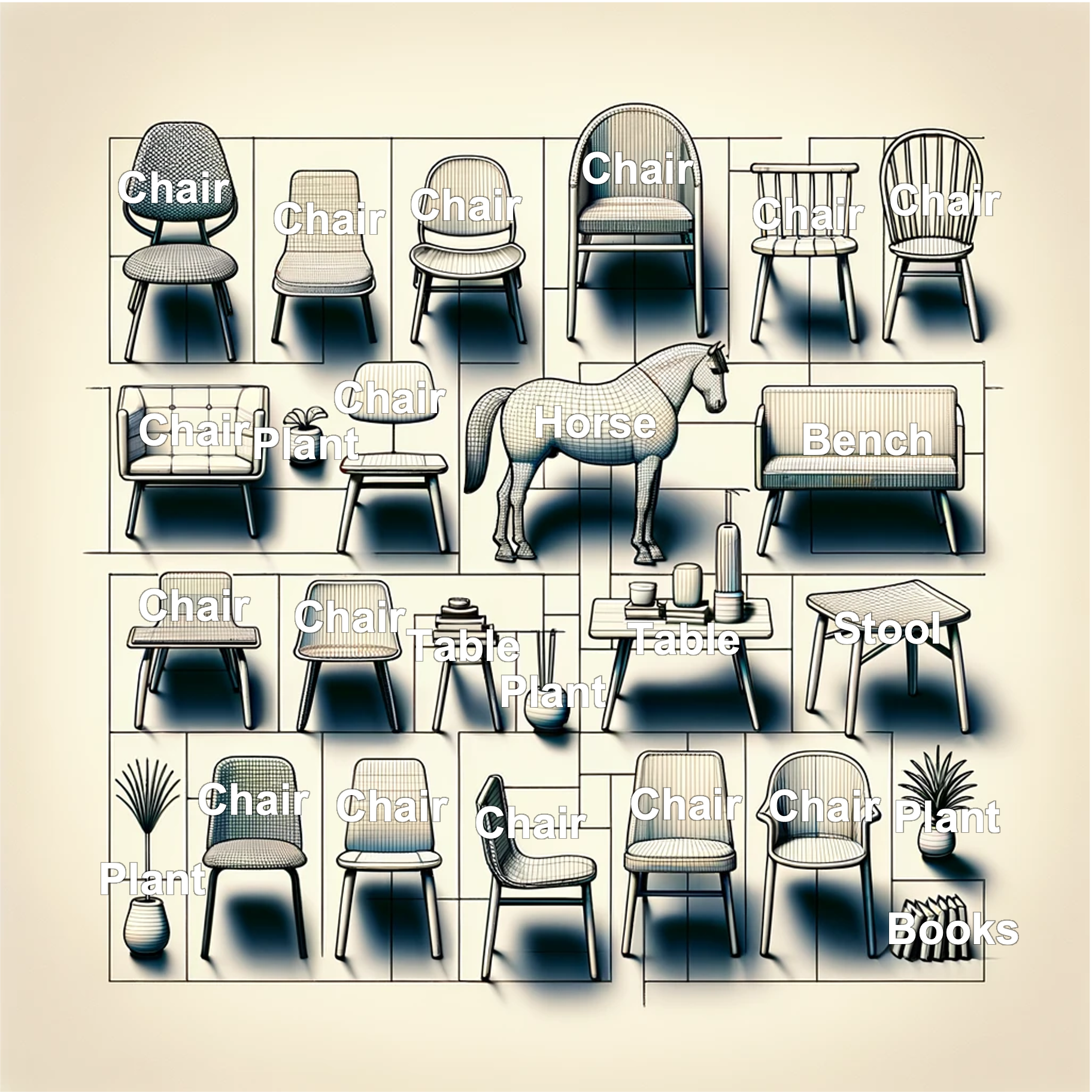
The data used for classifiers is labeled, meaning we have examples of objects along with their corresponding category labels. For instance, a dataset might contain images of chairs and non-chairs, each labeled accordingly (e.g., chair, horse, table, plant).
Mathematically, we can represent a dataset as a set of tuples:
where:
\(D\) is the dataset containing \(n\) labeled examples,
\(x^{(i)}\) represents the \(i\)-th input (e.g., an image or feature vector),
\(y^{(i)}\) represents the \(i\)-th label (e.g., “chair” or “horse”).
Binary Classification#
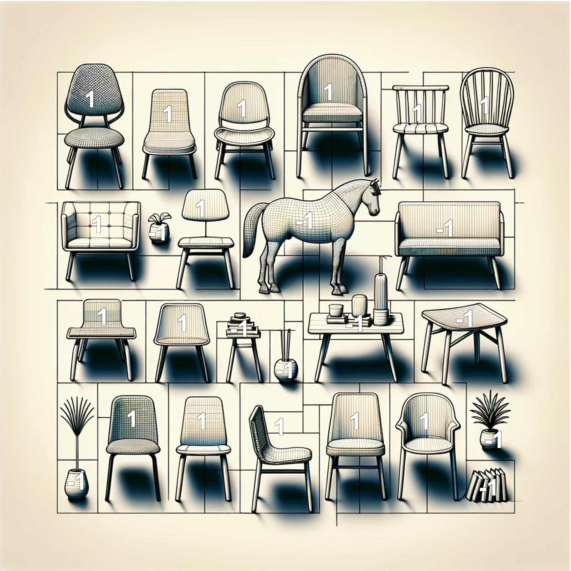
Here, we will specifically introduce binary classifiers. That means we do not want to classify objects into chairs, horses, tables, and plants. Instead, we are only interested in whether something is a chair or is not a chair.
We can express this by defining the label as either \(-1\) or \(1\):
where
Caveat: Feature Representation#
In the above example, we do not actually classify chairs themselves. Instead, we classify pictures of chairs. In this case, we can use black-and-white images as their feature representation. For instance, \(x^{(i)}\) could be a 2D vector of brightness values.
More generally, we need a function \(\varphi\) that transforms the “real thing” \(x\) into a feature representation \(x^{(i)}\):
The feature representation typically consists of list of numbers (vectors or tensors). To keep things short and concise, in this guide, we will primarily work with the feature representation instead of the “real thing” and will sometimes use \(x\) when we actually mean \(x^{(i)}\). However, it is important to note that using a poorly chosen \(\varphi\) can undermine even the most sophisticated learning algorithm.
Solution Space - Hypothesis Class#
Before finding a specific solution to a given problem, machine learning first requires defining a space of possible solutions. This space is often referred to as the solution space, hypothesis class, or hypothesis space. A single element of this space is called a hypothesis, and a hypothesis that (best) solves the problem is called a solution.
If you come from a different field, you can think of this as architectural constraints or inductive biases. More formally, the hypothesis space is defined as a parameterized function:
where a specific function \(y\) is given by:
where \(\theta\) represents the parameters of the function.
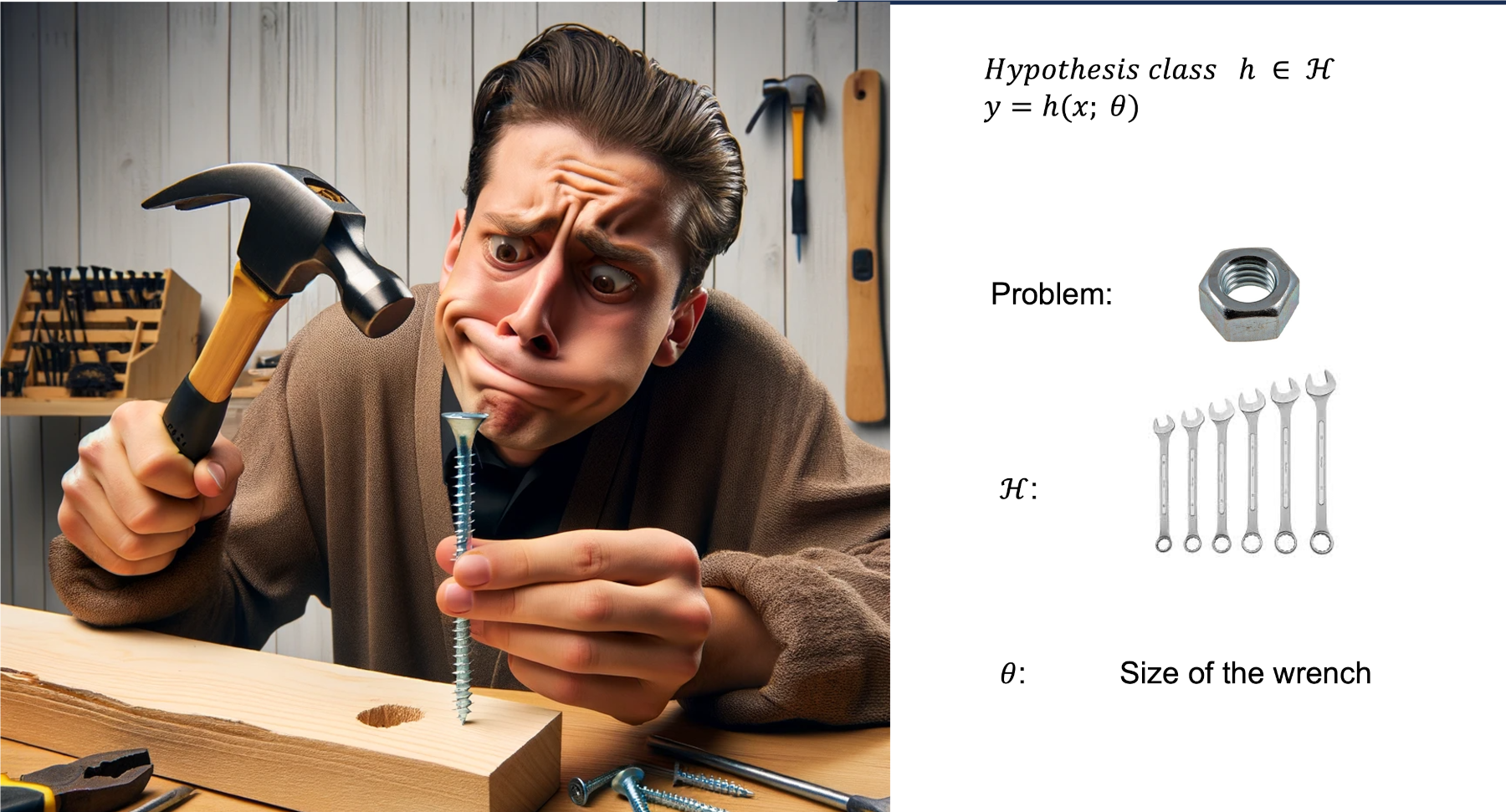
If you’re having a hard time wrapping your head around this concept, consider the following analogy:
Imagine you need to tighten a nut. A very broad hypothesis class would be all tools in my shed. However, this is too general, and searching through every possible tool would be inefficient. Instead, you can constrain the hypothesis class to all wrenches. Now, finding the right tool becomes much easier because you’ve eliminated irrelevant options.
Additionally, narrowing down the hypothesis class makes it easier to parameterize your choice. Instead of searching through every tool type, you now only need to adjust one parameter—the size of the wrench.
Note: In this example, you could even use a form of gradient descent (we will formally introduce this later) to find the correct wrench size:
If the wrench is too big, try a smaller one.
If the wrench is too small, try a bigger one.
By iteratively refining your choice, you are guaranteed to find the correct solution—provided that the right wrench is available in your shed.
Evaluating a Hypothesis: The Loss Function#
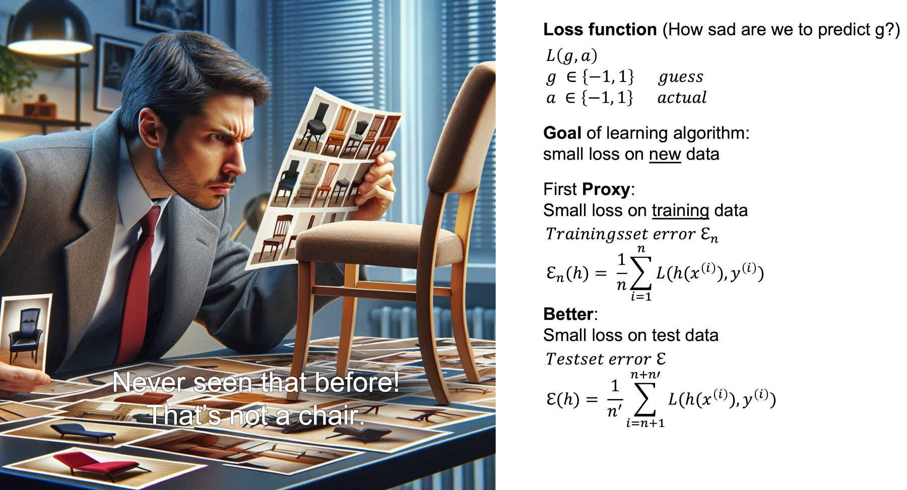
To evaluate a specific guess \(h\) from the hypothesis space \(\mathcal{H}\), we introduce the concept of loss. Essentially, loss quantifies how bad a given hypothesis \(h\) is at making predictions—it answers the question: How unhappy are we with the answer that \(h\) provides?
Given:
\(a\) as the actual label at \(x\),
\(g\) as the prediction made under the hypothesis \(h\),
our loss for a specific \(x\) is represented as a function \(L(g, a)\) (or $L(h(x), a). Often, the total loss over all data points is expressed as a average of individual losses.
A key principle in designing loss functions is that we are typically happy when ( g = a ), meaning our prediction is correct. The loss function should reflect this by assigning lower values when predictions are accurate and higher values when they are incorrect.
However, in this guide, we will not delve into regularization functions in detail.
Caveat: Don’t Overfit#
Loss functions make it clear that our goal is to minimize loss—we certainly don’t want a high loss. However, there are some important subtleties to consider:
Do we want to minimize the loss function only on the training data?
After all, the function we are searching for shouldn’t just perform well on the data it has already seen and that we have already labeled. If that were the goal, we could simply store all known labels in a dictionary and be done with it.
But how can we evaluate loss on data that the model hasn’t seen and that we haven’t labeled? That seems impossible, right?
To address this, we use proxies:
Training Loss (Training Error):
The first proxy is the loss computed on the training data:\[ \epsilon_n = \sum_{i=1}^{n} L(h(x^{(i)}), y^{(i)}) \]This helps guide the learning process by nudging the hypothesis in the right direction.
Test Loss (Test Error):
The second proxy is the loss on a holdout set, which consists of labeled data that we intentionally do not show the model during training:\[ \epsilon_{\text{test}} = \sum_{i=n+1}^{n'} L(h(x^{(i)}), y^{(i)}) \]
This serves as a better approximation of the model’s performance on unseen data, especially if our dataset is representative and not biased.
For example, a bias could be introduced if our dataset consists exclusively of furniture from IKEA. In that case, even when evaluating on a test set, we would still be testing only on IKEA furniture. As a result, the model might perform well on this specific subset but fail to generalize to chairs from other brands, leading to misclassifications. This would cause our classifier to perform significantly worse on truly unseen data compared to what the test loss suggests.
Note: Overfitting refers to a model that performs well on training data but significantly worse on test data. This occurs when the model learns patterns that are too specific to the training data, rather than generalizing to unseen examples.
Linear Classifiers#
Dataset \(D\)#
Let’s consider a dataset where \(x^{(i)}\) are vectors in d-dimensional space and labels are either \(-1\) or \(1\):
where
and
Hypothesis Space \(\mathcal{H}\)#
We can then define our hypothesis space \(\mathcal{H}\) as following:
where
and
Why does this work?
To build an intuition, let’s consider \(\theta_0 = 0\). Then, we need to determine the sign of the dot product:
In other words, when is the dot product between two vectors positive or negative? The dot product measures how much one vector aligns with another. Specifically:
The dot product is positive when the angle between the two vectors is less than \(90^\circ\).
The dot product is zero when the two vectors are perpendicular (in other words equal to \(0^\circ\)).
The dot product is negative when the angle is greater than \(90^\circ\).
Generalizing This to Decision Boundaries
This same intuition applies to any linear classifier:
The decision boundary is defined by the equation:
\[ \theta \cdot x = 0 \]This represents a hyperplane (a line in 2D, a plane in 3D, etc.) that is orthogonal to \(\theta\).
Any point \(x\) on the same side as \(\theta\) satisfies:
\[ \theta \cdot x > 0 \]Meaning it is classified positively.
Any point on the opposite side satisfies:
\[ \theta \cdot x < 0 \]Meaning it is classified negatively.
Any point exactly on the boundary satisfies:
\[ \theta \cdot x = 0 \]Meaning it is perpendicular to \(\theta\) and is neither positively nor negatively classified.
Try different theta vectors in the following graph to build an intuition (you can grab and drag \(\theta\)):
Loss L#
We define a simple loss:
In other words, we are sad if we guessed wrong (\(g \neq a\)) and not sad otherwise.
Learning Algorithm 1: Dumb learning#
For a given dataset \(D\), a learning algorithm that searches over the hypothesis space \(\mathcal{H}\) and tries to find a solution \(s \in \mathcal{H}\) that minimizes the Loss \(L\).
As a first try, let’s do dumb_learning: We randomly pick a number of \(\theta\) and \(\theta_0\) and pick the best:
dump_learning(D, k):
for j = 0 to k:
\(\theta^{(j)}\) = \(\text{random}(\mathbb{R}^d)\)
\(\theta_0^{(j)}\) = \(\text{random}(\mathbb{R})\)
\(j^{*}\) = \(\text{argmin}_{\{0, ..., k\}}(\epsilon_n(\theta^{(j)}, \theta_0^{(j)}))\)
return \((\theta^{(j^{*})}, \theta_0^{(j^{*})})\)
Note: The \(k\) in the above algorithm is what is typically referred to as a hyperparameter. It is not part of the parametrization of the hypothesis space but influences the learning. Here, the higher \(k\), the lower the loss, and one can even prove that:
meaning that if \(k\) grows larger and larger, eventually the loss will be zero for all points (if a solution exists, meaning there is some line that separates the points).
See dumb_learning in action:
Learning Algorithm 2: Clever Algorithm by a Clever Person#
1957 – Frank Rosenblatt, a very clever person whom some refer to as the father of deep learning, developed clever_learning, which he dubbed the Perceptron. It was later proven to solve all linearly separable problems—classification problems that can be perfectly separated by a hyperplane.
clever_learning(D, T):
\(\theta\) = \(0\); \(\theta_0\) = 0
for j = 0 to T:
for i = 0 to n:
if \(y^{(i)}(\theta \cdot x^{(i)} + \theta_0) \leq 0\):
\(\theta = \theta + y^{(i)} * x^{(i)}\)
\(\theta_0 = \theta_0 + y^{(i)}\)
return \((\theta, \theta_0)\)
Watch clever_learning in action! (You may want to restart the simulation a few times—this algorithm is so clever that it often finds the correct solution on the first try!)
Machine Learning as Optimization#
Clever Learning Algorithms for not so clever people

Here, we don’t want to rely on being as clever as the “father of deep learning” each time we have a new problem. Instead of using our intuition to come up with cool learning algorithms, we turn our problem into an optimization problem and use general purpose methods to find an optimum.
An optimization function is characterized by an objective function: \(J(\theta)\). The optimization then finds \(\theta^* = \text{argmin}_{\theta}(J(\theta))\).
A typical machine learning objective function is
with the training error
and a regularize term (for example to penalize large entries for \(\theta\))
The upside of framing a problem as an optimization problem, is that we can then use general purpose algorithms to optimize. For example, gradient descend:
Gradient Descend#
Imagine you are lost in the mountains and thirsty. How would you go about finding a water source? One strategy is to always take the steepest downward path at each step. This way you will find a lower point (the lowest local point) where the chances are high that there is water. This is exactly how gradient descent works in optimization problems. In nature, a river naturally follows gradient descent.
Intuition
Gradient descent is an iterative optimization algorithm used to find the minimum of a function. It follows these steps:
Start at a random point: Choose an initial guess for the solution.
Compute the gradient: The gradient (vector of partial derivatives) points in the direction of the steepest ascent.
Take a step in the opposite direction: Move against the gradient by a small step size (learning rate).
Repeat until convergence: Continue iterating until the function value stops changing significantly.
Types of Gradient Descent
Batch Gradient Descent: Uses the entire dataset to compute the gradient.
Stochastic Gradient Descent (SGD): Uses a single random data point per update.
Mini-Batch Gradient Descent: Uses small subsets of the data for each update.
1 Dimensional Gradient Descent#
Let’s first assume both \(\theta\) and \(f(\theta)\) are 1-dimensional (scalars). The update rule for gradient descent then is defined by
with \(f'(\theta_t)\) the derivative of \(f\) at point \(\theta_t\) and the learning rate \(\eta\).
We can also write this as an algorithm:
GD1D(\(\theta_{init}\), \(f\), \(f'\), \(\eta\), \(\varepsilon\)):
\(\theta^{(0)} = \theta_{init}\)
\(t = 0\)
loop
\(t = t + 1\)
\(\theta^{t+1} = \theta^t - \eta f'(\theta^t)\)
until \(|f(\theta^{(t)}) - f(\theta^{(t-1)})| < \varepsilon\)
return \(\theta^{(t)}\)
To get a better intuition, here a few examples:
Note: For a convex function, it can be shown that for each error \(\varepsilon\) no matter how little, one can find a learning rate \(\eta\) so that the above algorithm converges. In mathematical terms:
where \(f(\theta^*)\) is the minimum value of \(f\).
n Dimensional Gradient Descent#
The above algorithm works just as well when \(\theta\) has more than one dimension. Instead of the derivative \(f'\), we then use
Note: Here, the output of \(f\) is still one-dimensional. You can imagine this, for example, as a height map when \(\theta\) is two-dimensional. Then, the gradient will be the steepest direction—the opposite direction of the fall line. If you like to ski, this is the line where you are “drawn to,” or, similarly, the path where water will naturally flow downhill.
Logistic Regression - Why?#

Why Linear Classifiers are not Optimal (nor Optimizable\(^*\))#
In the above section about linear classifier, we defined an error function. Why can we not just plug that into our gradient descent function?
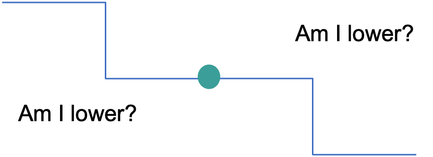
Again, imagine you are lost and thirsty in the mountains. But since you have learned about gradient descent, you have a solution, right? Just follow the opposite of the gradient. What do you do if you reach a plateau though (in other words the gradient is 0)? If you are a very committed to the gradient descent algorithm you will die from thirst in this scenario.
The same is true for our linear classifier. There are “plateaus” everywhere. You can convince yourself by “wiggling” the \(\theta\) vector in the interactive plot earlier. Small changes will not change the amount of blue or red dots which means small changes wouldn’t change our error function (the amount of dots classified incorrectly). In other words, our gradient is zero and the gradient descent algorithm doesn’t know in which direction to go.
\(^*\) At least not with the standard gradient descent algorithm described earlier.
To build up an intuition, you can think about this as: Certain properties of the loss function make it easier to optimize it. Steps are problematic, continuity is good.
Why don’t we really on the Perceptron then?#
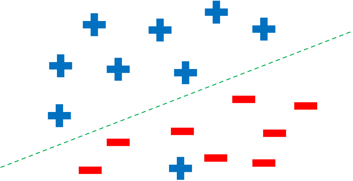
The perceptron only guarantees that a solution is found if (and only if) the minimum loss of the function is zero. Then it will find the solution. However, we would also like to find the best solution (the one that optimizes the loss) in other scenarios like this:
Linear Logistic Classifier#
Note
Until now, we used the labels (-1, 1), but to make things easier, we will change the labels to (0, 1).
Hypothesis Class \(\mathcal{H}\)#
The only difference between a linear classifier and a linear logistic classifier is that instead of the \(sign\) function, we now use \(\sigma\):
Our hypothesis will look like this (here to make things explicit we name the hypothesis LLC instead of \(h\)):
with
The following image might help with your intuition why this is a reasonable function to choose:
Remember the linear classifier hypothesis:
This can be understood as a “step function”:

Remember the linear logistic classifier hypothesis:
This can be understood as a smoother version of the same “step function”:

Note: By now, if you have built some intuition about gradient descent you should also have an intuition why a smoother version of the step function might be easier to optimize: Instead of a error function with plateaus, we will build an error function that is “smooth”.
Loss function \(L\)#
With our hypothesis space \(LLC\), we can now define a Loss function \(L\):
Let’s look at our prediction \(g\):
this can be interpreted as the probability of guessing that the label at \(x^{(i)}\) is \(1\). But then, we can write the accuracy of the hypothesis \(A\) on the training set as:
this is the probability of guessing the full training set (every label) correctly.
A more compact way of writing this is:
Tip 1: This trick of using exponentiation to replace conditional branching is a powerful and elegant technique. It’s particularly useful in optimization and gradient-based learning because it allows for smooth, differentiable computations without explicit if statements. It works since \(a^0 = 1\) and \(y^{(i)}\) is either 0 or 1. Convince yourself, that the formulas are equivalent by trying out both cases of the if statement (\(^{(i)} = 0\) and \(^{(i)} = 1\)).
Tip 2: \(A\) is also called the Bernoulli likelihood function.
With all the math involved in defining a loss function, it’s easy to lose sight of the main goal: providing an objective function that can be optimized using gradient descent (or similar methods).
What Really Matters?
Most of the time, we don’t necessarily care about the interpretability of the loss function. Instead, we only need to ensure that:
The loss function provides meaningful gradients that guide the optimizer toward better model parameters.
Optimizing the loss improves the model’s performance.
For example, if we take an objective function \(O\) and multiply it by a positive scalar, the function itself becomes “stretched.” However, this does not change the location of the minima and maxima—it only scales the gradients. Since gradient-based optimizers adjust step sizes accordingly, optimization results remain unchanged.
Thus, while a scaled loss function might lose its original interpretability, it still leads to the same optimal solution when used in training.
This is not only true for stretching but for all monotonic transformations: If we preserve the order of the values, that means we use a transformation \(w\) for witch \(x_i < x_j \implies w(x_i) < w(x_j) \ \forall x_i, x_j\), then our gradient descent optimization still gives the same results.
This is important, since we will use now log-transform \(A\) to get our final loss function \(A'\)
This is not only true for stretching but for all monotonic transformations:
If we preserve the order of the values, that means we use a transformation ( w ) for which:
We used:
\(\log(a*b) = \log(a) + \log(b)\)
\(\log(a^b) = b * \log(a)\)
Since we want to maximize \(A\), we can minimize -\(A'\) which is also called Negative log likelihood or cross entropy:
We won’t go through the full derivation of the gradient of \(\mathcal{L}\) with respect to \(\theta\) here, but it’s a great exercise for those interested. Tip: Use the chain-rule.
The final result for the gradient is:
Caveat: Linear Separability#
The linear logistic classifier only gives good answers when the data is linear separable. To get around this we can sometimes transform our data, for example by using an additional dimension and a polynomial basis:
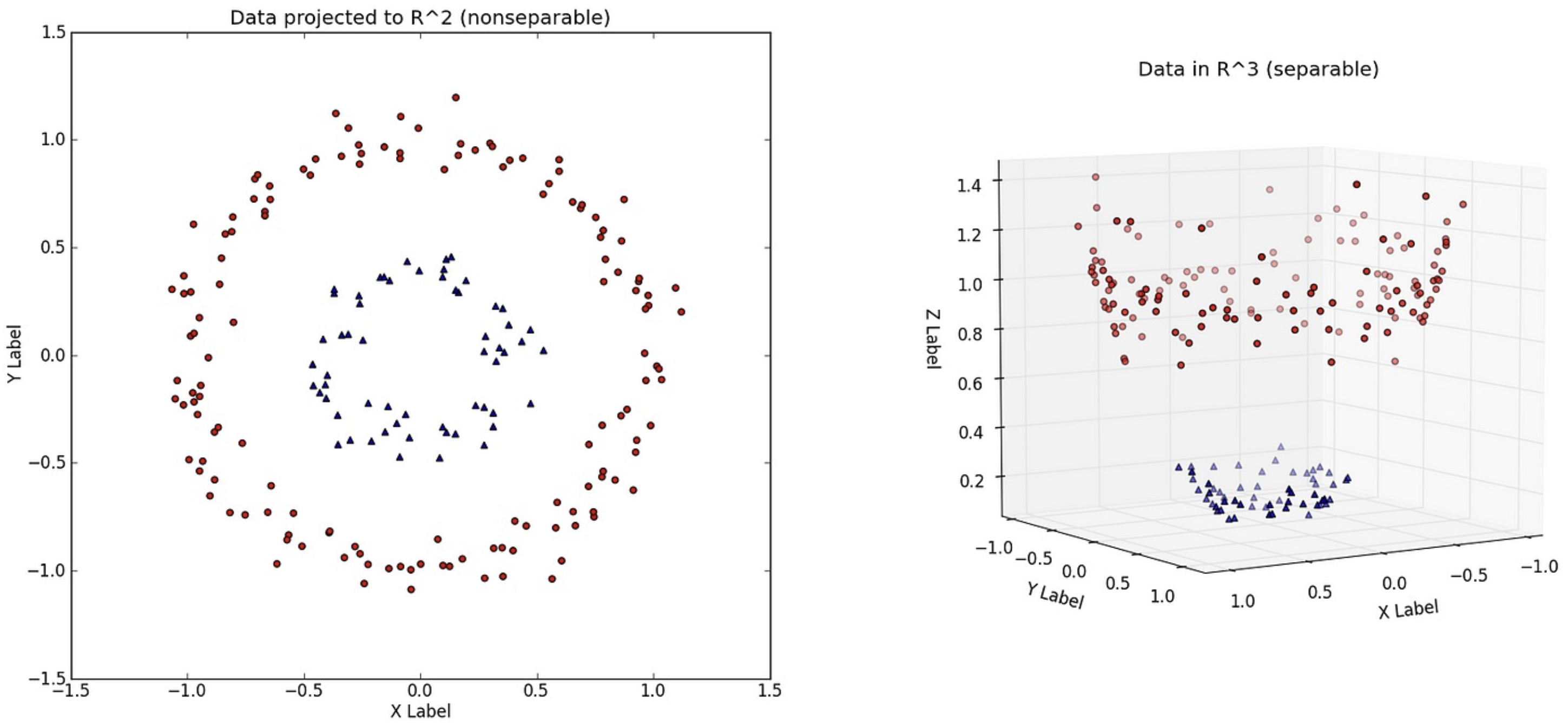
However, a neural networks provide a more general solution for this problem:
Neural Networks#
Neuron#
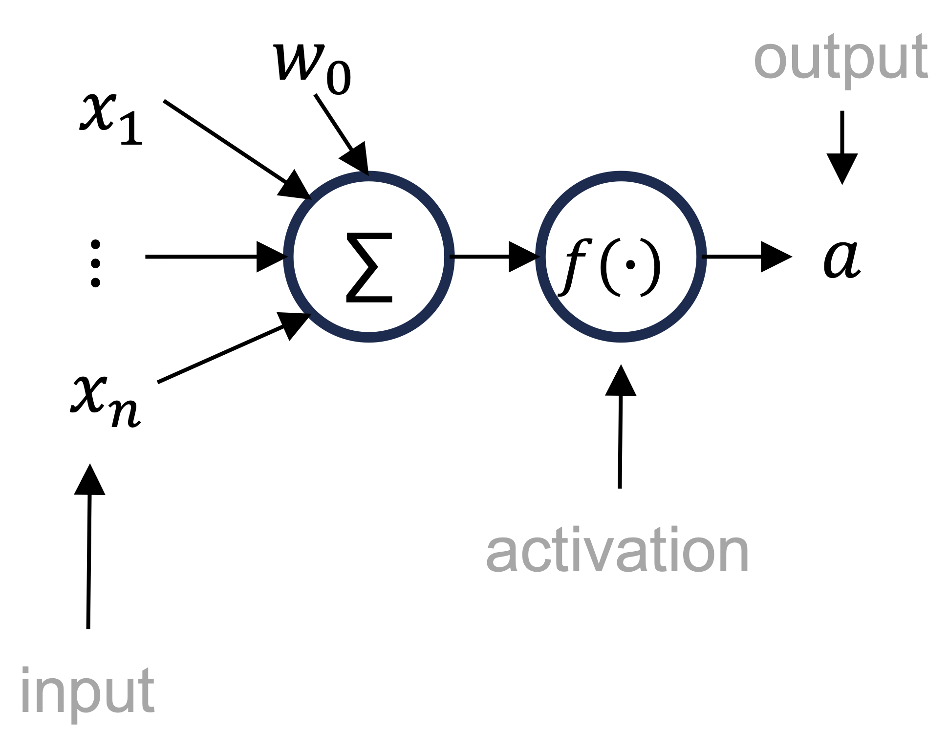
A single neuron in a neural network computes its activation using a weighted sum of inputs \(\vec{x}\)), followed by a activation function \(f\). Mathematically, this can be written as:
or in vector notation
Note:
If \(f = sign\) this is just a linear classifier.
If \(f = \sigma\) it is a linear logistic classifier.
Layer#
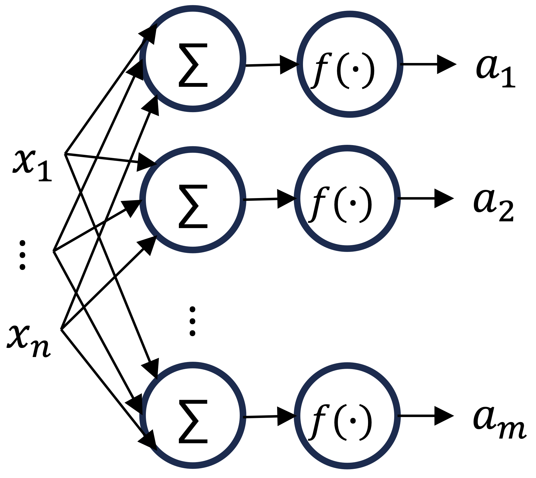
We call \(m\) parallel neurons a layer of size m.
we can write this as
or more concise in matrix form:
with
Network#

A neural network is when we (serially) connect multiple layers
Note: If \(f^L = \sigma\) and \(W^L \in \mathbb{R}^{\cdot \ \text{x} \ 1}\), the neural network is a (logistic) classifier.
Activation Functions#
Think about what could be “good” activation functions \(f^i\)?
To keep things simple, let’s consider linear activation functions \(f(z) = \lambda * z\).
If all our activation functions are linear, we can write:
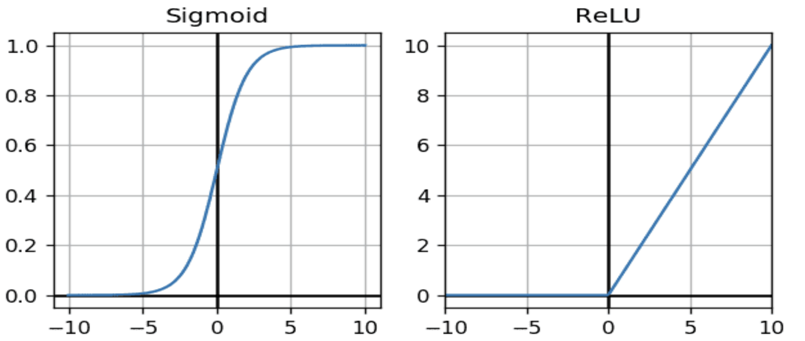
in other words, we can write our neural network as one layer and the matrix \(W^total\)! This is defeats the purpose of using multiple layers. Instead, activation functions are only helpful if they are non-linear. In addition, for reasons we explored in the section about optimization, they should be differentiable (that means step functions or signs are not ideal). But, we can use \(\sigma\) or ReLU:
Backpropagation#
If you’ve been following along, understanding backpropagation seems almost trivial. In essence, backpropagation is just a more fancy word for the chain rule you are familiar with from calculus.

with:
\(\frac{\delta loss}{\delta A^L}\) defined by the chosen loss function
\(\frac{\delta A^L}{\delta Z^L} = (f^{L})'\)
\(\frac{\delta Z^L}{\delta W^L} = A^{L-1}\)
And, we can then successively calculate the Losses for each weight by:
with
\(\frac{\delta Z^i}{\delta A^{i-1}} = W^i\) since \(W\) are linear functions
\(\frac{\delta A^i}{\delta Z^i} = (f^i)'\)
which we can both easily calculate.
THANK YOU AND HAPPY CODING!
